In this post, we will estimate the parameters defining a CIR process from a (simulated CIR) dataset. We will then use antithetics to estimate an expectation dealing with the Heston model, where the underlying volatility is modeled by a CIR model.
Let ![X=(X_t: t \in [0,T])](https://s0.wp.com/latex.php?latex=X%3D%28X_t%3A+t+%5Cin+%5B0%2CT%5D%29&bg=ffffff&fg=333333&s=0&c=20201002) be a stochastic process such that
be a stochastic process such that  where
where  is a standard Brownian motion. (Note: this is the CIR process, commonly used to model interest rates.)
We arbitrarily select values for the parameters: 
Now, we run set.seed(19870210) and generate a sample path of  in R, storing the simulated values for in mydata.
R Code
Henceforth, we pretend that the process  with some specific but unknown parameters has generated the data.
FACT: 
Using this, we write a function to estimate  from the data. We obtain
R Code
Next, let  where
where  is the Lamperati transformation for . That is:
  Then,
Then,  is a stochastic process such that

where is a standard Brownian motion, and  is a function. Its density (for the interval
 ![[0,T]](https://s0.wp.com/latex.php?latex=%5B0%2CT%5D&bg=ffffff&fg=333333&s=0&c=20201002) ) is given by
) is given by

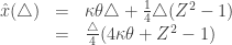
Now define a function  as the following:

Then:

It then follows that the density  of is specified by:

We can now estimate the parameters  in R by maximizing the likelihood
R Code
Running the code, we estimate  to be
to be 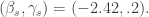 Remember that these values are inferred from the data set we created by creating a realization of a CIR process. Since we know the real values of the underlying process to be
  we expect that if we ran this experiment
  (large) times (i.e. simulate the CIR process times and estimate
  times),
We will reference the following paper on simulating a Heston model, where the underlying volatility (instead of the interest rate is modeled by a CIR model.
A paper
In particular, consider the following basic Milstein scheme:


Claim: this scheme has a positive probability of generating negative values of  and therefore cannot be used without suitable modifications.
Proof: Let  Then,
Then,
Thus, will clearly be negative when 
Let  be such that
  and
and  (a CIR process). Now define
  We will (with our estimated parameters) use the antithetic method and (10) to estimate
  by simulation.
We wish to simulate 2 processes  that are identically distributed and negatively correlated. To do this, we first simulate 2 processes
  that are identically distributed and negatively correlated using (10), the Milstein equation.
Next then obtain the processes  and from there,
  trivially.
Recall that we wish to estimate . We calculate  . Taking
  we obtain a sample value
  . To estimate , we repeat this simulation times, and
R Code
After running this experiment with our parameters  , we obtain
  Looking more closely at our data, we see that (indeed)

Let us inspect a realization of  :
:
 This is what we expect (mean reversion at 0.2). Let us now see the Heston process that was adapted from this realization.

Recall that (or rather, infer from  )
) 
 is a strictly positive process that hovers around its mean. For the sake of illustration, we can (roughly) think of as
  . Then obviously, is a log-normal process, so this plot is what we would expect.
In summary, despite our uninteresting result for  we have shown how to estimate the parameters defining a CIR process from a (simulated CIR) dataset, and how to use antithetics to estimate an expectation dealing with the Heston model, where the underlying volatility is modeled by a CIR model.